Which Distribution Best Captures the Gap in Continuous Time

What is the Gamma Distribution?

The gamma distribution is a continuous probability distribution that models right-skewed data. Statisticians have used this distribution to model cancer rates, insurance claims, and rainfall. Additionally, the gamma distribution is similar to the exponential distribution, and you can use it to model the same types of phenomena: failure times, wait times, service times, etc.

The most frequent use case for the gamma distribution is to model the time between independent events that occur at a constant average rate. Using this distribution, analysts can specify the number of events, such as modeling the time until the 2nd or 3rd accident occurs. In this context, reliability analysts use the gamma distribution to model failure times.

The gamma distribution is a generalization of the exponential distribution. The gamma distribution can model the elapsed time between various numbers of events. Conversely, the exponential distribution can model only the time until the next event, such as the next accident.

Related posts: Understanding Probability Distributions and Skewed Distributions

Gamma Distribution Parameters

There are two versions of this distribution. The three-parameter gamma distribution has three parameters, shape, scale, and threshold. When statisticians set the threshold parameter to zero, it is a two-parameter gamma distribution. Let's see how these parameters work by graphing the probability density function for this distribution!

To determine which probability distribution best fits your data, read my post Identifying the Distribution of Your Data.

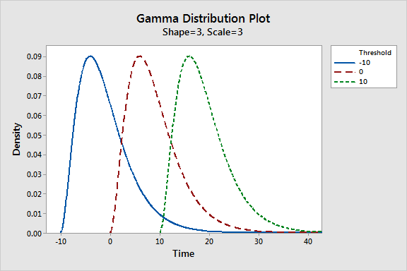
Threshold Parameter

The threshold defines the smallest value in a gamma distribution. Some analysts refer to this parameter as the location. All values must be greater than the threshold. Negative threshold values allow the distribution to handle both negative and positive values. Zero lets it have only positive values. A two-parameter gamma distribution simply has the threshold set to zero.

Holding the shape and scale parameters constant, the threshold shifts the distribution left and right. In the probability distribution plot below, I show the threshold's effect in action!

Shape Parameter (α)

The shape parameter for the gamma distribution specifies the number of events you are modeling. For example, if you want to evaluate probabilities for the elapsed time of three accidents, the shape parameter equals 3. Shape must be positive, but it does not have to be an integer. Statisticians denote the shape parameter using alpha (α).

The plot below shows how changing the shape parameter affects the distribution while holding the other parameters constant.

Notice how increasing the shape causes the elapsed times to increase. That makes sense because, keeping everything else constant, you'd expect the length of time to grow when you increase the number of events. For example, three accidents (α = 3) will take longer to occur than one (α = 1), and five (α = 5) takes longer than 3.

For very high shape values, the gamma distribution approximates the normal distribution, as shown below.

When the shape of a gamma distribution is an integer, it is known as an Erlang distribution. Analysts frequently use the Erlang distribution in queuing theory.

Scale Parameter (β)

The scale parameter for the gamma distribution represents the mean time between events. Statisticians denote this parameter using beta (β).

For example, if you measure the time between accidents in days and the scale parameter equals 4, there are four days between accidents on average.

Rate Parameter (λ)

Alternatively, analysts can use the rate form of the scale parameter, lambda (λ), for the gamma distribution. Lambda is also the mean rate of occurrence during one unit of time in the Poisson distribution. Use the following equations to convert between the scale (β) and rate (λ) forms:

• β = 1 / λ
• λ = 1 / β

They are reciprocals. To understand why let's return to our example of one accident occurring every four days on average (β = 4). An equivalent way to state it is that an average of one-quarter accident occurs during one day (λ = 1 / 4 = 0.25).

Effect of Changing the Scale on the Gamma Distribution

The scale parameter represents the variability present in the gamma distribution. Higher values cause the distribution to expand further right and decrease the height. Conversely, lower values contract the distribution to the left and increase its peak.

Alternatively, if you use the rate form of the parameter, higher rates shrink the distribution while lower rates spread it out.

The relationship between the scale parameter and the spread of the gamma distribution makes sense when you understand that the scale represents the mean time between events. When the time between events is longer, the probabilities for prolonged times logically increases. In the graph below, I illustrate this by modeling probabilities for the 4th event (shape = 4) and varying the average times between events.

This graph looks similar to the chart comparing shape parameters. While increasing the shape and scale parameters will both extend the elapsed times, the shape parameter can genuinely change the shape in ways that the scale cannot. For instance, the shape parameter can change the distribution so it looks like the exponential and normal distributions. The scale parameter can only stretch out the distribution that the shape defines.

Related post: Measures of Variability

Comparing the Gamma Distribution to Other Distributions

The gamma, exponential, and Poisson distributions all model different characteristics of a Poisson process. A Poisson process has independent events occurring at a constant mean rate. All these distributions can use lambda as a parameter, which represents that average rate of occurrence. Here's how these three distributions compare.

The gamma distribution models the time between events. Time is a continuous variable, and the gamma distribution is, likewise, a continuous probability distribution. Conversely, the Poisson distribution models the count of events within a set amount of time. A count is a discrete variable and the Poisson distribution is a discrete probability distribution.

The gamma and exponential distributions are equivalent when the gamma distribution has a shape value of 1. Remember that the shape value equals the number of events and the exponential distribution models times for one event. Therefore, a gamma distribution with a shape = 1 is the same as an exponential distribution.

For example, a gamma distribution with a shape = 1 and scale = 3 is equivalent to an exponential distribution with a scale = 3.

Related posts: Poisson Distribution and Exponential Distribution

jameschumake85.blogspot.com

Source: https://statisticsbyjim.com/probability/gamma-distribution/

Share this post